Manual for Familias 3
Daniel Kling 1
(daniel.l.kling@gmail.com)
Petter F. Mostad 2
(mostad@chalmers.se)
ThoreEgeland 1,3 (thore.egeland@nmbu.no)
1Oslo University Hospital
Department of Forensic Services
Oslo, Norway
2Mathematical sciences
Chalmers University of Technology and Göteborg
University
Göteborg, Sweden
3 Norwegian University of Life Sciences
Department of Chemistry, Biotechnology and Food Science
Aas, Norway
Last edited: 2017-02-01
Contents
1 Introduction 6
2 Example – a preview of Familias 7
2.1 Calculation of the
likelihood ratio (LR) by hand 8
2.2 Calculation of the
likelihood ratio using Familias 9
3 User’s guide 14
3.1 General DNA data 15
3.2 Import system data
from file 16
3.3 Export system data to
file 17
3.4 Options 17
3.5 Specifying mutation
models 18
3.6 Persons  20
20
3.7 Known relations  22
22
3.8 Case related DNA data  22
22
3.9 Import case data 24
3.10 Compare
data 26
3.11 Pedigrees
 26
26
4 DVI module 31
31
4.1 Add unidentified
persons 31
4.2 Add reference family 33
4.3 Evaluate reference
families 38
4.4 Search 39
5 Blind Search  42
42
5.1 The blind search 42
5.2 Viewing merged
profiles 44
6 Simulation interface 46
7 Familial searching 49
7.1 Profiles/Persons 50
7.2 Search options 51
7.3 Search 52
8 Advanced options 54
9 Create
database 57
10 Export
to R-Familias 58
11 Plotting 59
12 Error handling and input checking 60
13 A Appendices 61
13.1 A1
Theory and methods 61
13.2 A1.1
Prior model 61
13.3 A1.2 Posterior
model 62
13.4 A1.3
Subpopulation corrections 63
13.5 A1.4
Mutation models 64
13.6 A2
Solved excercises 70
13.7 A3
Generating pedigrees automatically 70
13.8 A4
Implementation of prior distribition 71
13.9 A5
Description of general input files for Familias 73
13.10 References 78
i Preface
This document updates the documentation of the Familias software
available at http://www.familias.no (previous versions can be
found at http://familias.name) in connection with the 3.2 version released in
February 2017. A complete list of changes and bug fixes appears on the home
page. Additional material (lecture notes, exercises with solutions, videos
etc.) are available at http://familias.name/book.html. Comments on the
documentation or the program can be sent to daniel.l.kling@gmail.com.
The book by Egeland, Mostad and Kling ((Egeland, Kling et al. 2015)contains
complete details of the mathematical models and also provide more background
and context to applications suited for Familias. Please help us
improving this manual by sending suggestions whenever you cannot find an
adequate description of the features.
A new section has been added (11) to cover some error
handling and input checking performed by Familias.
ii News
Familias 3 (version 3.0 and above) includes a
disaster victim identification module (DVI). In addition a blind search feature
is implemented. Moreover a completely new interface to perform simulations is
included. All is described in this manual.
Version 3.1.6 (and above) includes a Familial searching
interface, briefly described in this manual. Several updates have been made so
make sure to use the latest version. The paper (Kling and Füredi 2016)
reports some real applications of Familias searching resulting in some
serious crime cases being solved.
There is a separate software, FamiliasPedigreeCreator,
freely available at http://www.familias.no (Download section) capable
of preparing an R-script in turn producing plots for all Familias
projects in a specific directory (and sub-directories). The plots are stored
into png files that can be displayed in the software (version 3.2 and above) or
inserted into a report.
iii Supported
platforms
Familias runs on all Windows environments (tested on
XP, 7, 8 and 10). For Mac users try a Windows emulator environment, see this site
listing some commonly used emulators. Similar for users of other OS, the
software should run on all Windows emulators.
The Familias program may be used to compute
probabilities and likelihoods in cases where DNA profiles of some people are
known, but their family relationship is in doubt. Given several alternative
family trees (or pedigrees) for a group of people, given DNA measurements from
some of these people, and given a data base of DNA observations in the relevant
population, the program may compute which pedigree is most likely, and how much
more likely it is than others. Obviously, there are several other programs
performing similar tasks. As far we know a distinguishing feature of Familias
is its ability to handle complex cases where potential mutations, silent
alleles and population stratification ( -corrections) are accounted
for, together with its ability to handle multiple pedigrees simultaneously. The
program has been validated (Drabek 2009).
The books(Buckleton, Triggs et al. 2005)and
(Balding 2005)provide
a general background to forensic genetics.
-corrections) are accounted
for, together with its ability to handle multiple pedigrees simultaneously. The
program has been validated (Drabek 2009).
The books(Buckleton, Triggs et al. 2005)and
(Balding 2005)provide
a general background to forensic genetics.
The original reference to Familias is (Egeland, Mostad et al. 2000)
whereas (Kling, Tillmar et al. 2014)
describes Familias 3. Several example data files, are available
from the site http://familias.name.
Online help including a short tutorial, is available directly from the
help-function of the program.
Familias has been applied in a large number of cases,
including identification following disasters, resolving family relations when
incest is suspected and determining the most probable relation between a person
applying for immigration and claimed relatives of the individual.
The contents of this document are as follows. Section 2
gives a brief introduction to program by means of a simple worked example.
Next, Section 3
provides an overview of the options available in the program, along with
suggestions for typical values for the various parameters. Some more theory and
advanced options are presented in Appendix A1. Appendix A2contains
links to old (Familias 2 or 1.97) and new (Familias 3) exercises
with solutions. Appendices A3
and A4
describe advanced options. Finally, the file format of the input file is
described in detail Appendix A5; this is only relevant for programmers
as the purpose is to enable programmers to write code producing input files for
the Familias program, on the “Familias format”. There is open R version
of the core of program http://cran.r-project.org/web/packages/Familias/
which facilitates extensions.
Regarding transferring data from GeneMapper® to Familias,
Antonio Vozmediano (a.vozme@hotmail.es)and Lourdes Prieto (lourditasmt@gmail.com)
have developed GeneMapperToFamilias which provides an alternative
to more generic functionality described below. NB, Familias now accepts
exported genotypes from GeneMapper as well.
This section presents a very simple case. First, calculations
are done by hand and then we demonstrate how the calculations are done using Familias.
We consider the following hypotheses concerning the
relationship between a manAF and Child:
·
H1: AF is the father of Child
·
H2: AF is not the father of Child
An illustration of the
hypothesised relationship is given in Figure 1. The mother is undisputed. Such
illustrations denote men with squares and women with circles (Bennett, French et al. 2008).
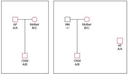
Figure 1. The pedigree
corresponding to hypothesis H1 (left) and H2 (right)
The allele frequencies of A and B
are and Hardy-Weinberg equilibrium
is assumed. The child has inherited the allele B from his mother and the allele
A must be inherited from the father.
and Hardy-Weinberg equilibrium
is assumed. The child has inherited the allele B from his mother and the allele
A must be inherited from the father.
The likelihood ratio is then given by
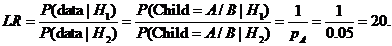
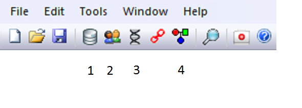
Figure 2. The main menu of
Familias
The standard calculations in Familias are performed
by going through the four steps indicated in Figure 2.
1. General DNA data. The window appearing after
clicking  should be completed as shown in Figure 3 (only ‘manual’ is entered to indicate the database used; this has no impact
on calculations).
should be completed as shown in Figure 3 (only ‘manual’ is entered to indicate the database used; this has no impact
on calculations).
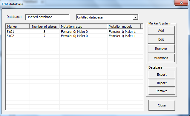
Figure 3. The General DNA data
window.
2. Allele system. The window appearing after clicking
Add should be completed as shown in Figure 4.
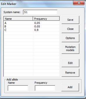
Figure 4. The Allele System window.
3. Persons. The window appearing after clicking  should be completed as shown in Figure 5 below.
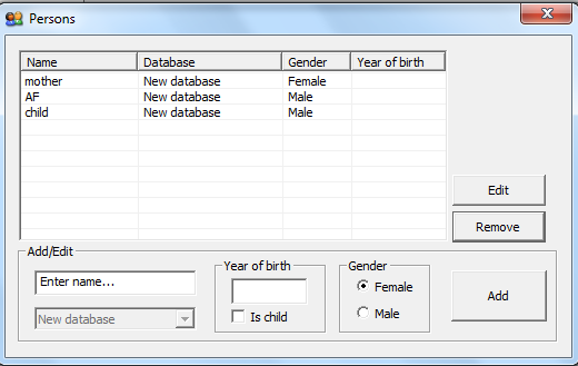
Figure 5. The Persons window.
4. Case related DNA. The window appearing after
clicking  should be completed as shown in Figure 6below.
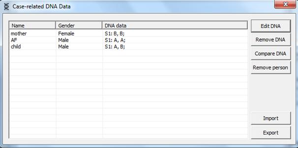
Figure 6. The Case related DNA
window.
The data is entered by clicking the persons and using the
menus.
4. Pedigrees. Click . First the pedigree
corresponding to hypothesis H2 is entered by clicking Add. This should be completed
as shown in Figure 7.
. First the pedigree
corresponding to hypothesis H2 is entered by clicking Add. This should be completed
as shown in Figure 7.
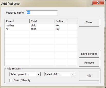
Figure 7. Defining the pedigree
corresponding to hypothesis H2.
The next pedigree is defined similarly. The answer, LR =
20, appears by clicking Calculate
, results shown in Figure 8.
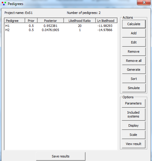
Figure 8. The result as shown
in the Pedigrees window.
3
User’s guide
In this section we explain how to use the Familias software
with more details on the functionality. The main menu of Familias is
illustrated in Figure 9below.

Figure 9. Main menus of
Familias
The first four buttons are common to most windows programs: New file, Open file and Save file.. The next five
buttons are specific to Familias and will be treated in the following
sections. They are General DNA data, Persons,
Case related DNA,
Known relations, and Pedigrees
. These buttons will make a window with the same title appear. In addition,
there is functionality to do Blind search, and there is a DVI module
 . All windows can be accessed through
the Tools (or File) menu where appropriate shortcuts can be found.
. All windows can be accessed through
the Tools (or File) menu where appropriate shortcuts can be found.
Usually, the user will go through
some of the options in a particular fashion. First, the allele systems are
defined under General
DNA data (defining a population frequency database). This is sometimes done manually, but it is also possible to
import such data from a database file (more common in case work). Secondly, the
persons are defined by their name, gender and age under Persons (age is not
mandatory). Next, under Case Related DNA Data, the genotypes of the relevant persons are entered for all
or a subset of the available allele systems. Possible known relationships are
entered under Known
Relations. This last functionality is only
used to save time in cases where some relationships should be fixed for all
pedigrees and is therefore not really needed. Finally, the Pedigrees window is used to define pedigrees (either manually or
automatically), and perform calculations of probabilities and likelihoods.
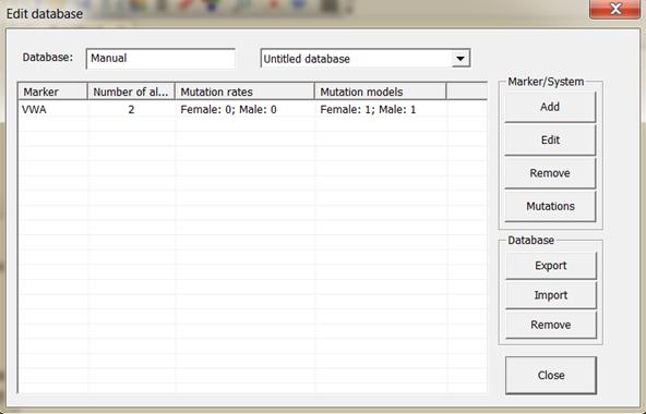
Figure 10. A system may be
added, edited or removed manually.
3.1 General
DNA data
This window provides options for adding, editing, removing,
reading and writing allele systems/markers. An illustration of the window is
given in Figure 10. Systems may be edited manually or by reading files.
3.1.1
Entering data manually
To enter a new allele system manually, press Add. Then the Allele system window,
illustrated in Figure 11, appears. Here you enter the system name, the alleles
and their respective frequencies. It is recommended to ensure that the allele
frequencies sum to 1 (Familias will perform normalization if not). If
necessary, an extra allele, called say ‘Rest allele’ can be added as
demonstrated in Figure 11. A rest allele will be added automatically if the
frequencies do not sum to 1. A technical note is that Familias uses the limit
0.00000001. In other words, if the allele frequencies sum to 1.000000001 they
will not be adjusted.
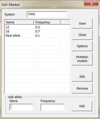
Figure 11. The window for entering an allele system.
3.1.2
Sorting
Alleles are sorted numerically according to name if
possible, otherwise alphabetically. This is essential when using mutation
models that depend on the ordering (the repeat number) of the alleles. Alleles
with a repeat number below 10 do not need to be modified with 0 as the first
digit in this version of Familias (In contrast to previous versions). If
the first character of an allele name is a letter, it is probably wise to use
small or capital letters consistently. For instance alleles a and E are sorted E,
a whereas a, e are sorted a, e.
The file below corresponds to the output from an Excel file,
with tabs as separators. The different systems are listed below each other,
separated by at least one blank line. The listing for each system starts with
the name of the system, followed by a number of lines, each containing the name
of the allele, and as the following item, the frequency. The alleles are sorted
by the program, numerically if possible, otherwise alphabetically according to
name, to correspond to the corresponding sorting when inputting alleles
manually. The data is read in, and is added to the current allele systems. The
name of the file read is recorded in the upper left corner adjacent to the
field Database. This field
can be edited to keep track of the database used or modified. If allele systems
with the same names already exist, these are replaced. The systems are created
with zero mutation rates and no silent alleles. If the frequencies listed are
not positive, an error is issued, and the reading of data stops. If the
frequencies do not add to 1, they are adjusted to do so, with a warning. An
example of input is given below.
Table 3.1: Example of system data that can be read
into Familias from the General DNA Data window. You can load the data
between the lines below by cutting and pasting in an editor like Word or Excel.
There should be a blank line before a new marker, i.e., before SYS2 below. It
is important that you save the data as a text file, from excel you should use
tab delimited text file, as mentioned previously. The allele frequencies of
SYS2 do not sum to 1. On reading into Familias a warning will be given
for this system before the allele frequencies are scaled to add to 1.
SYS1
A 0.002
B 0.096
C 0.119
D 0.225
E 0.326
F 0.163
G 0.056
H 0.013
SYS2
6 0.056
7 0.073
8 0.190
9 0.192
10 0.253
11 0.143
12 0.089
The system data can be written to a file on the same format
as used for input. If you have problems importing system data, it is a good
idea to first export data and check the file format.
Some settings for the allele system/marker is found in the Options
window, see Figure 12.
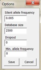
Figure 12. The window for changing allele system
options.
3.4.1
Silent alleles
It is possible to specify a frequency for a silent allele.
This refers to alleles that for some reason or other are not detected with the
common methods. With a positive silent allele frequency, you cannot know
whether an identified homozygote really is homozygote or if he is heterozygote
with the other allele being a silent allele. The silent allele frequency and
the other allele frequencies should add to 1. Further details on silent alleles
are given in the solved exercises, see Appendix A2.
3.4.2
Database size
This option specifies the database size of the marker. This
indicates the number of typed individuals that constitutes the populations
frequency database. The value may be different for different markers. The value
is used to compute frequencies of new (previously unobserved) alleles.
3.4.3
Dropout
Specifies marker specific dropout probability. Note, for
dropout to be active you have to specify at least one profile you wish to model
dropout for. This applies to kinship calculations, for dropout probabilities
connected to direct matching see Advanced settings.
3.4.4
Min. allele frequency
Specifies the minor allele frequency (MAF) for the current
marker. If a new allele is detected (or if an existing allele frequency is
changed) a warning will be given if the specified frequency is lower than the
MAF. The MAF may also be forced during the likelihood computations, see
Advanced settings. Allele frequencies below the stipulated minimum are
increased to the minimum value. The allele frequencies may then sum to more
than 1 and scaling is required before saving. After the scaling it may happen
that frequencies are slightly below the stipulated minimum.
The default value for mutation rates are zero. However, if
it is known or reasons to suspect that there is a non-zero mutation rate, it
should be specified here. A reasonable mutation rate could be around 0.005. The
program offers the possibility to distinguish between male and female mutation
rates. The reason for this is that paternal alleles tend to mutate more often
than maternal alleles. There are 5 different mutation models to choose from,
1)
Equal probability
(Simple)
2)
Probability
proportional to frequency (Stationary)
3)
Step-wise
(Unstationary)
4)
Step-wise
(Stationary)
5)
Extended step-wise
model (Unstationary)
A mutation model is defined by its mutation matrix. This
mutation matrix can be viewed using the File > Advanced > View Mutation
Matrix option. Mathematical details are provided in Appendix A1, along
with an example of analytical calculations for the various models. However, to
use the program all you really need to know regarding stationarity is the
following: If a model is stationary this implies that adding irrelevant persons
will not affect the result. Conversely, for unstationary models adding
irrelevant persons may lead to slightly different results.
For models 3, 4 and 5 the probability of mutation depends on
the size of the mutation.
For example, if you have an allele with 14 repetitions, this
allele will be more likely to mutate into an allele with 13 or 15 repetitions
than to an allele with 12 or 16 repetitions. For models3, 4 and 5, Familias the
user must supply a parameter. A typical Mutation
range is 0.1.This
value corresponds to a mutation probability that decreases by one tenth for
each additional unit length difference between the parent allele and the
offspring allele. Be aware that, for models 3 and 4, the “length” of the
alleles is only decided by the order in which they are entered. The difference
in length between two subsequent alleles is taken to be 1, which means that it
in some circumstances it will be necessary to enter unobserved alleles.
However, if using model 5, Extended
stepwise model, the length of the alleles are taken to be the actual
entered number. If using systems with base pair numbers as alleles (e.g. 300,
302 etc), this model will not work as intended. Then we should perhaps resort
to one of the other models.
Consider next model 2, Probability
proportional to frequency. Here the probability of mutating to an
allele is proportional with this allele’s frequency in the population. This
means that if you have, e.g., an allele A with frequency 0.05 and another
allele B with frequency 0.1, then the probability for a mutation leading to a
new allele B is larger than one resulting in a new allele A.
In the model Equal
probability (simple) the probability of mutating from one allele to
another allele is the same independently of the frequency and the range of the
alleles.
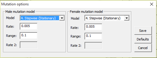
Figure 13. The mutation models
and parameter options.
3.5.1
Mutation model dialog
There is a special window available to apply mutation
parameters to all (or selected) systems at once. For instance to change the
models of all systems or the rates. The dialog is accessed via File >
Tools > Mutations. The dialog in in Figure 14 appears. The same options as in Figure 13 exist, but in addition a tick box to only change the models
are available. This may be useful to keep marker specific rates and ranges and
only change the models. In addition the user can choose to Apply to the
selected systems/markers or Apply to all systems (regardless of selections).
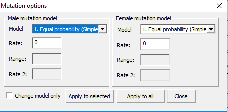
Figure 14. Mutation dialog.
3.6 Persons

By pressing this button, the window shown in Figure 15appears. Here you define the persons involved in the case. For each person a
name and gender must be specified. For most applications this is the only
information needed and used. In addition, it is possible to enter a year of
birth, and you may also specify if the person is a child or in effect has no
children. Concerning the year-of-birth specification: as Familias only
makes use of the relative dates, it is possible to use this option to specify
age differences even when the exact year-of-birth is unknown. The “Is Child”-option is used to
limit the number of possible pedigrees if the Generate
option of the pedigree window is used to generate pedigrees automatically.
Similarly, giving two persons the same year of birth also limits the number of
pedigrees as there will then be no parent-child relationships between these
individuals. The list of persons is edited by means of Edit (or double clicking an item in the list) and Remove.
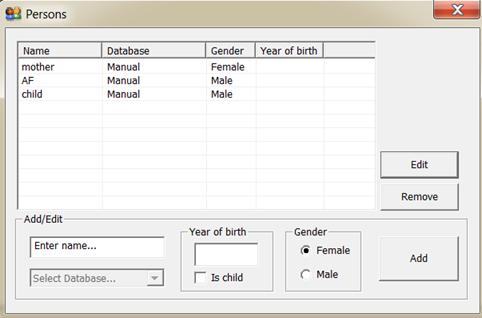
Figure 15. The window for entering the persons
involved in a case.
3.7
Known relations 
This is where known relations (fixed relations) are defined.
You are advised to avoid the functionality in Known relations unless you
intend to analyse a greater number of pedigrees. The functionality in this
section is never really needed; it only simplifies input when many pedigrees
are analyzed or generated.
If it is certain that, e.g., F is
the father of D, then this could be specified here. It is only possible to
define parent-child relations. This means that if, for example, two girls are
known to be sisters, this cannot be defined straightforward, but through their
relations with the common parents. The window is illustrated in Figure 16. The menu  is not strictly needed as this
information can be provided also when the pedigrees are defined. All relations
defined in the Known relations window will appear in all pedigrees.
is not strictly needed as this
information can be provided also when the pedigrees are defined. All relations
defined in the Known relations window will appear in all pedigrees.
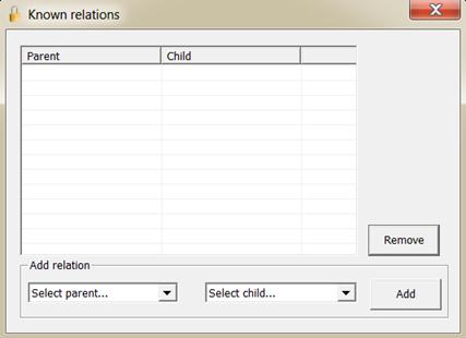
Figure 16. The window for entering known relations.
3.8 Case
related DNA data 
In this form you enter the DNA data for the persons for whom
this information is available. This can be done manually or by reading from a
file.
3.8.1
Manually
By marking one of the persons on the list in the window
shown in Figure 17, and pressing Edit
data, a new window appears (see Figure 18). Here you enter, for the
selected person, the DNA data of all the investigated allele systems. For
persons for whom there are no available DNA data, just leave it open. Apparent
homozygotes are entered with two of the same allele, also in the cases where
there could be silent alleles.
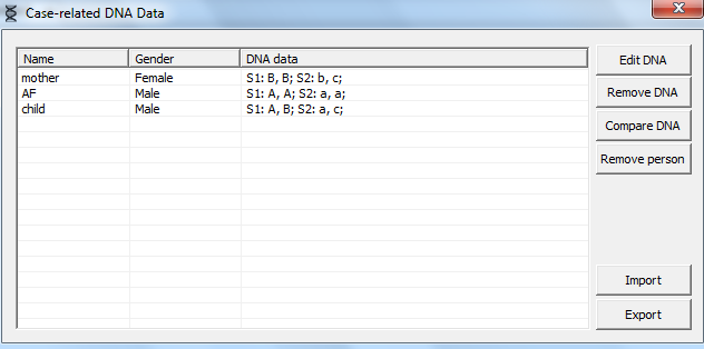
Figure 17. Selecting the
persons to assign genotype data is done in this window.
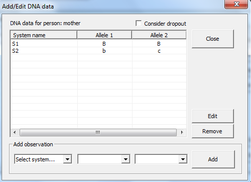
Figure 18. Adding DNA data for
a selected person is done in this window. By ticking Consider dropout
dropouts are considered. Note, you have to specify a dropout probability for
each marker system or specify a profile specific dropout probability in the Advanced
Data for specific samples can now also be read from files.
The data for specific samples can be given as a table. There are four different
format which can be read be Familias, listed below.
The format can be outputted
from Excel, using tabs as separators (from Excel, save as Text (Tab
delimited)). The table should have a line with headings and the following lines
should each represent a sample source, i.e., a person. Blank lines (i.e., lines
where there is nothing in the first column) will be ignored. The first column
should list the names of the sample sources, i.e., the persons. If the names
correspond to names of persons already entered, the data will be added to the
data for this person. Otherwise, the persons will be added as they are read
in. The data for the systems must be provided prior to reading case data.
There must be two columns specifying sex chromosomes in the table. These
columns must be beside each other, the first must contain the letter “X” as all
entries, and the second must contain either “X” or “Y”, depending on the sex.
(Remember that Familias is case sensitive. The X and Y should be in
capitals.) When new persons are added, they will be given the sex specified by
these columns. For existing persons, the data is ignored. Except for the three
columns described above, all columns must come in pairs of two, beside each
other, with the headings specifying the name of the allele system the columns
contain data for. The headings for each pair must be identical, except for the
last character (which could be, for example “1” and “2”). After the last
character has been removed, the remaining name (removing blanks at the end)
must correspond exactly to the name of an already entered allele system. The
two columns below then contain the names of the alleles observed in this
system, for the respective persons. Note that homozygotes must have alleles
entered twice, once in each column. Missing data are coded with a ‘*’. Both (or
none) alleles must be missing for a marker. An example of an input file is
given below.
Table 3.2:Example of case data that can be read
into Familias from the Case Related DNA Data window. The system
called SYS1 and SYS2 must be given on beforehand, for example by reading the
data of Table 3.1 above. The names (na1, na2 and Jakob) may or may not be
given. The loading of the data is explained previously.
|
Name
|
Amel 1
|
Amel 2
|
SYS1 1
|
SYS1 2
|
SYS2 1
|
SYS2 2
|
|
Na1
|
X
|
X
|
F
|
G
|
8
|
9
|
|
Na2
|
X
|
Y
|
G
|
G
|
10
|
11
|
|
Jakob
|
X
|
Y
|
G
|
G
|
9
|
10
|
3.9.1.2
Tab separated (With commas between alleles)
The format can as previously
be outputted from Excel, using tabs as separators (from Excel, save as Text
(Tab delimited)). The table should have a line with headings, and the following
lines should each represent a sample source, i.e., a person. Blank lines (i.e.,
lines where there is nothing in the first column) will be ignored. The first
column should list the names of the sample sources, i.e., the persons. If the
names correspond to names of persons already entered, the data will be added to
the data for this person. Otherwise, the persons will be added as they are read
in. The data for the systems must be provided prior to reading case data.
There must be one columns specifying sex chromosomes in the table. For each
person there must be either a X,X or X,Y in the specific column. When new
persons are added, they will be given the sex specified by these columns. For
existing persons, the data is ignored. For each system we have only one column
where the header must correspond exactly to the name of an already entered
allele system. The column below then contains the names of the alleles observed
in this system, for the respective persons with a separating comma between the
alleles. Note that homozygotes must have alleles entered twice. Missing data
are coded with a ‘*’. Both (or none) alleles must be missing for a marker. An
example of an input file is given below.
Table 3.3:Example of case data that can be read
into Familias from the Case Related DNA Data window. The system
called SYS1 and SYS2 must be given on beforehand, for example by reading the
data of Table 3.1 above. The names (na1, na2 and Jakob) may or may not be
given. The loading of the data is explained previously.
name amel SYS1 SYS2
na1 X,X F,G 8,9
na2 X,Y G,G 10,11
Jakob X,Y G,G 9,10
The analyzed data from
GeneMapper should be outputted as shown in Table 3.4 below. The table should
have four headings, with the order, Sample name, Marker name, Allele1 and
Allele2.This can easily be specified creating a Table setting named Familias,
e.g., where the Genotype tabs have exactly the specified setup. The first
column should list the names of the sample sources, i.e., the persons. (Note
that the same name may be listed on several rows, see Table 3.4) If the names
correspond to names of persons already entered, the data will be added to the
data for this person. Otherwise, the persons will be added as they are read in.
The data for the systems must be provided prior to reading case data. There
must be one rows specifying the sex chromosomes, i.e. the gender of the person
in the table. When new persons are added, they will be given the sex specified
by these columns. For existing persons, the data is ignored. For each system we
have only one row where the second column of the row must correspond exactly to
the name of an already entered allele system. The next two columns then contain
the names of the alleles observed in this system.
Table 3.4:Example of case data that can be read
into Familias from the Case Related DNA Data window. The system
called SYS1 and SYS2 must be given on beforehand, for example by reading the
data of Table 3.1 above. The names (na1, na2 and Jakob) may or may not be
given. The loading of the data is explained previously.
Name marker allele1 allele2
na1 amel X X
na1 SYS1 F G
na1 SYS2 8 9
na2 amel X Y
na2 SYS1 G G
na2 SYS2 10 11
Jakob amel X Y
Jakob SYS1 G G
Jakob SYS2 9 10
3.9.1.4
CODIS xml format
Familias provides functionality to import data on the
CODIS xml format. This file format is described elsewhere. One of the main
point of this import function is the ability to easier exchange data between
labs, as the CODIS format is fairly standardized. In addition Familias
can import exported data from the CODIS software, exported to xml files (cmf
format).
In later versions of Familias, a Compare DNA
button has been added. This button makes it easier to compare genotypes of
several persons (if several persons are selected). If only one person is
selected, 1/RMP, i.e., 1 divided by the random match probability, is
calculated, see Figure 19. The user can convert this to the RMP. For the below
example,
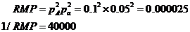
This calculation of RMP assumes Hardy-Weinberg equilibrium
unless the kinship/theta parameter is non-zero.
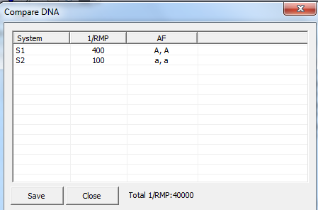
Figure 19. The compare DNA
dialog, displaying the random match probability for a profile with two typed
markers.
3.11 Pedigrees 
In this form you may add your own pedigrees or you may use Familias
to generate pedigrees, this latter option is discussed in Appendix A3. After
having generated the pedigrees, one can calculate probabilities and likelihoods
ratios and produce reports. In the following we will go through the set of
buttons and options of the window shown in Figure 20starting in the upper right
corner.
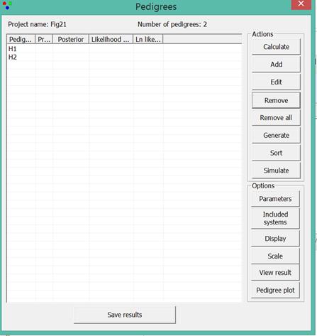
Figure 20. The Pedigrees window
with two defined pedigrees.
Calculate
This button performs the calculations
Add: Creating pedigrees
Usually, the first thing to do is to create a set of
pedigrees manually by clicking Add.
The pedigree is defined by giving the parent child relations as
exemplified in Figure 21. The Extra persons button is used to
introduce individuals needed to define a pedigree. For instance, such extra
persons may be needed to define cousin relations. There are various examples of
pedigrees Available from http://familias.name/book.html.The pedigree name can
be edited. Note that a relation can be defined as being direct/identity. This
implies that the two samples/individuals are assumed to be from the same
sample/individual and calculations are performed based on this assumption. For
instance, for monozygotic twins the two individuals have a direct/identity
relation in one of the hypotheses whereas a full sibling relation is defined in
the alternative hypothesis. An R script for plotting in R is generated by Plot in R.
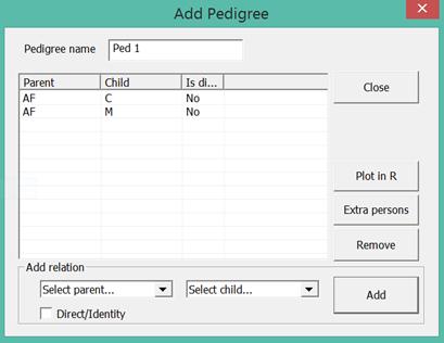
Figure 21. AF is defined as the
father of C and M. C and M are thus half-sibs. An extra parent is needed to
define full sibs.
Edit: Editing pedigrees
The pedigrees are edited using this button.
Remove
This button is used to remove all selected pedigrees.
Remove all
This button is used to remove all pedigrees.
Generate: Generate pedigrees automatically
See Appendix A3.
Sort
The results are sorting in according to decreasing LR.
Simulate
Starts the simulation interface, explained in Section 3.8.
Parameters
Various parameters can be set. The most frequently used is
the kinship parameter ( ). The
remaining parameters are explained in Appendix A4.
). The
remaining parameters are explained in Appendix A4.
Included systems
By default all systems are used for calculation. This option
can be used to extract results for selected systems.
Display
Select what to display in the pedigree window. (Prior,
Posterior, LR and ln likelihood).The natural logarithm displayed, i.e., ln can
be converted to log10 by log10(x)=ln(x)/2.303
Scale
Select the pedigree to scale against, used when calculating
LR.
View result
Select a pedigree and press to see genotypes and LR for all
markers. This is a new functionality introduced in Familias 3 that can
be used to detect for instance mutation. The dialog appears in Figure 22, and there is most likely a mutation for the marker PENTA_E
Pedigree plot
Plots generated and saved as png files can be viewed along
with the genotypes. The function is used in combination with the FamiliasPedigreeCreator
software, mentioned in Section 10.
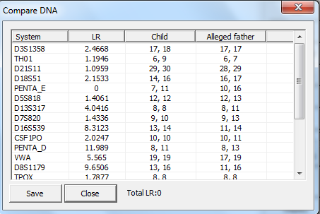
Figure 22. View of the results
(LRs) for individual markers.
Save results
Brings up the Report dialog where results can be saved using
several options
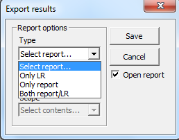
Figure 23. Creating a report.
Only
LR just gives precisely only the LR (total). Next format (rtf,
csv, xml or txt) can be selected and finally the extent of detail (Simple, Moderate, Complete).
4
DVI module
Disaster victim identification is a term describing the
event where a number of unidentified samples are compared with a number of
reference samples, commonly with known origin. The latter could be personal
belongings such as profiles from tooth brushes etc., while it is also common to
obtain data from relatives of the missing person, so called reference family
members.
The DVI module is divided into three steps, first adding the
unidentified individuals/samples and their genotypes, second the reference
families and the alleged pedigrees and last the DVI search. There are also
several functions that may be additionally carried out in each step, see below
for detailed description.
Open the DVI interface by clicking the button , or
from Tools > DVI module > Add Unidentified Persons. By pressing
this button, the window shown in Figure 24appears (Note, the exact appearance
may vary slightly depending on what version of the Familias you are
using).
For each person/element/remain a name and gender must be
specified. See below for a description of each button.
Edit person
Edit the general
information for a person such as gender and name.
Edit DNA
By marking one of the persons on the list, in the window
shown in Figure 1, and pressing Edit data, a new window appears (see Figure 25). Here you enter, for the selected person, the DNA data of all the
investigated allele systems. For persons for whom there are no available DNA
data, just leave it empty. Apparent homozygotes are entered with two of the
same allele, also in the cases where there could be silent alleles. More
commonly we import genotype data from file, see below.
Remove
Removes the
selected persons from the list.
Move
Used to place an
individual in a reference family (after or before identification).
Sort
Sorts the list
alphabetically by ID.
Compare
By selecting one (or more) of the persons in the list in Figure 24and pressing Compare, a comparative view of the
person's DNA will appear.
Search selected
Includes only the
selected persons in the DVI search. The selected list is only stored for one
search and is restored upon returning to this window.
Blind search
Opens up the blind
search interface for the list of unidentified persons. NB! Not used to blindly
compare the unidentified remains with the reference families. Such
functionality is described in Section 4.4 below.
Import/Export
Imports/Exports
data.
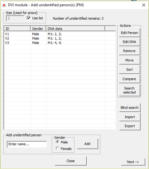
Figure 24. The Add unidentified
persons window for entering the persons involved and their genotypes.
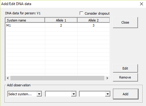
Figure 25. Adding DNA data for
a selected person is done in this window.
Once the persons are defined in the Add unidentified
persons window click Next (or click Add Reference
Families from Tools >
DVI
module.
See below for a comprehensive description of each of the
buttons on the dialog that appears, see Figure 26 for an illustration.
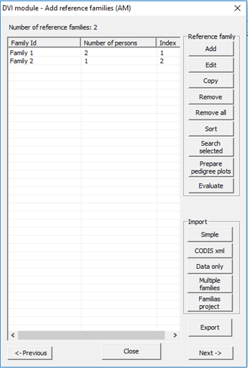
Figure 26. Window for defining
and importing reference families.
Add
Adds a new family. Define the persons in each family in the
window illustrated in Figure 27, and specify the relation between the
individuals in the family and the missing person in the pedigree window shown
inFigure 28. The buttons appearing in the figure are more or less
self-explanatory. The button Check may be used to check the pedigrees
for any inconsistencies/mutations.
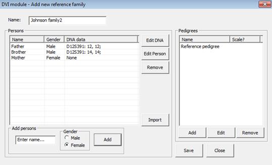
Figure 27. Adding persons to
the family and their genotypes is done to the left in this window, the
pedigrees are generated by clicking the Add button to the right in the window. The
‘Reference pedigree’ in the upper right part is always included by default to
include the possibility that a victim belongs to none of the families.
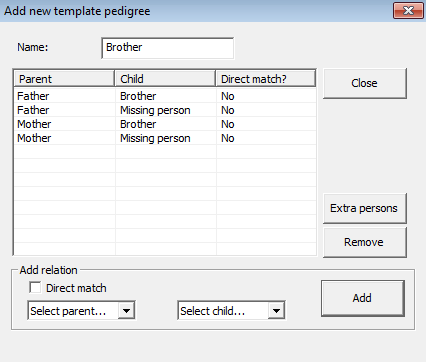
Figure 28. Defining a pedigree
in the DVI module. The individual named Missing person is used to indicate a
link to each of the unidentified person in the subsequent search.
Edit
Open the selected family for edit.
Copy
Copy a selected
family including persons and pedigrees. Useful to define several missing
persons within the same family.
Remove/Remove all
Remove selected
families.
Sort
Sorts the list
alphabetically by ID.
Search selected
Includes only the
reference families in the DVI search. The selected list is only stored for one
search and is restored upon returning to this window.
4.2.1
Prepare pedigree plots
This feature is new in Familias 3.2 and will create
an R-script for the selected reference families. Running this R-script will
generate plots for all the selected families and store them in a folder
connected to the DVI project. The plots may be viewed outside Familias
or using the Evaluate feature described next
4.2.2
Evaluate
This will open a new dialog to evaluate the selected
reference families. See detailed description in Section 4.3 below.
4.2.3
Import data from file
For larger DVI cases or missing person operations it is
convenient to import data from a file instead. Familias supports a
number of different formats, described below.
Simple
This format
corresponds to the normal Familias format, described in Section 3.9.1.1. A (optional) relationship indicator may precede
the line describing the data for the person. Familias will try to automatically generate the pedigrees.
All imported families should be checked such that the relationships have been
correctly identified. See Table 3.5 for a comprehensive list of relationships.
See below for file format.
|
Sample id
|
D12S391 1
|
D12S392 2
|
|
[Brother]
|
|
|
|
Per
|
12
|
14
|
CODIS xml
The CODIS xml
format is a format used in the CODIS software and also by some other systems.
The format is described elsewhere but allows for simple transfer of data. Familias can easily read a complete export file from the
CODIS software and can interpret some standard relationships.
Data only
Similar to the
Simple format but in this file an additional column describing the family id
(preceding sample id) is included. This makes it in turn possible to include also
several reference families in a single file. See below for file format:
|
Family id
|
Sample id
|
D12S391 1
|
D12S392 2
|
|
Family 1
|
Per
|
12
|
14
|
|
Family 2
|
Daniel
|
13
|
14
|
|
|
|
|
|
The following
format should also be accepted:
|
Family id
|
Sample id
|
D12S391
|
|
Family 1
|
Per
|
12,14
|
|
Family 2
|
Daniel
|
13,14
|
Multiple families
Same as the
previous format but in addition include a column (preceding sample id),
describing the relationship, see Table 3.5.
See below for file
format:
|
Family id
|
Relationship
|
Sample id
|
D12S391 1
|
D12S392 2
|
|
Family 1
|
[Brother]
|
Per
|
12
|
14
|
|
Family 2
|
[Father]
|
Daniel
|
13
|
14
|
Familias project
Recognizes and imports files
on the standard Familias (.fam or .txt) format. Imports persons and
pedigrees as well as known relations. Extra persons are turned into ordinary
family members. Recognizes the identifier "missing person" or
"MISSING PERSON" as the missing person.
Table 3.5: Relationships recognized by Familias
|
Relationship
|
|
[Brother]
|
|
[Sister]
|
|
[Sibling]
|
|
[Father]
|
|
[Mother]
|
|
[Parent]
|
|
[Son]
|
|
[Daughter]
|
|
[Child]
|
|
[Aunt]
|
|
[Uncle]
|
|
[Niece]
|
|
[Nephew]
|
|
[Half-sister]
|
|
[Half-brother]
|
|
[Grandmother]
|
|
[Grandfather]
|
|
[Direct]
|
|
[Identity]
|
4.3 Evaluate reference families
The functionality described here relates to the dialog in
the DVI module (Add Reference Families > Evaluate).
The dialog is a versatile tool to thoroughly evaluate the performance of each
of the reference families in an identification. The dialog below will appear.
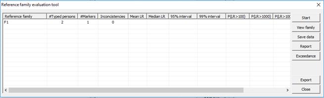
Figure 29. Reference family evaluation interface.
All selected reference families are listed. The following
also appears in the table,
1. Number
of typed persons (information on which markers not provided)
2. Number
of typed markers (combined for all typed persons in the family)
3. Number
of inconsistent markers (can be used to locate persons/markers that may cause
problems in the search)
4. Summary
statistics parameters (mean/median, intervals, exceedance probabilities,
exclusion probability) that will be available once simulations have been
performed, see below.
The buttons are described below.
4.3.1
Start
Pressing Start will initiate a simulation
process. The window below will appear with some options. Selecting Conditional
simulations will cause Familias to generate an R script. This script
may be run in R making use of the library fam2r, which is a wrapper for
the library paramlink, to conditionally simulate data. In short this
simulation approach uses the available genotypes (i.e. typed reference family
members) to obtain summary statistics.
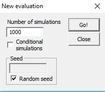
Figure 30. Starting a new evaluation/simulation.
4.3.2
View family
Brings up a view to watch the pedigree (provided plotting
has been done using functionality described previously in the section “Prepare
pedigree plots”) as well as genotypes and any inconsistent markers.
4.3.3
Save data
This function will save the raw LR output from the
simulations. Useful to further study the reference families.
4.3.4
Report
This will generate a report for the families with all the
results from the evaluations. Not yet implemented.
4.3.5
Exceedance
This will export exceedance probabilities for a range of
thresholds. Useful for plotting and other purposes.
4.3.6
Export
Writes all the elements of the displayed table to a text
file.
When the persons and pedigrees in each family are defined
click Next
(or click Search
from Tools
> DVI module.
The functions, see Figure 31is described below.
Search
Perform a search. It is recommended to save all changes
before conducting the DVI search. Prior to the search, a dialog will ask for a
match threshold, pick 0 (zero) to obtain results for all comparisons. NB! If
the Quick search feature is enabled in the Advanced dialog (which
is default), only matches with less mismatches (i.e. markers with
inconsistencies) will be reported, see also Section Advanced options8.
Quick scan
Performs a quick scan. This option brings up the blind
search interface, see Figure 32, and will blindly search the reference family
members against the unidentified persons using specified parameters. In other
words, this function disregards any specified family relations and performs a
blind search. The scan will perform pairwise matching, i.e. each family member
is tried separately against each unidentified person. This will mitigate
problems resulting from unknown “false” relationships in the reference
families.
Sort
Sorts the match list. The user selects the sort key.
Apply threshold
Apply a new LR threshold, possibly decreasing the number of
matches in the list.
Display
Select what columns to display in the match list.
View match
View the specifics of a match, i.e., the LR for individual
markers.
Confirm match
Confirms a match and create a report on a specific match. In
addition it is possible to move an unidentified person to a reference family
thus effectively removing him/her from the list of unidentified individuals.
Remove
Remove a selected match from the list.
Create report
Create a comprehensive report of the search. The same
options as described in Section 3.11 are available when creating the report.
Export list
Exports the list to a tab-separated text file. The file can
be easily edited and manipulated in a software such as Excel.
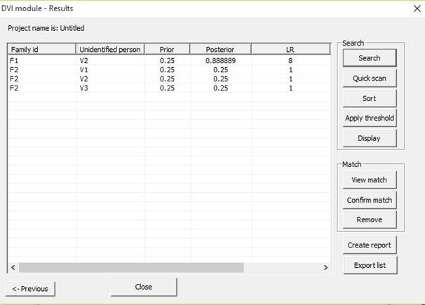
Figure 31. The results from a
DVI search. Both LR and posterior probability are displayed.
5
Blind Search
The Blind Search module is a new tool (in Familias 3)
used to perform an unspecific relationship search for a set of person with some
DNA data. Consider for example a list of persons with DNA data for which we
want to know about any undefined relations. Using the module we may perform a
search for any of the relationships, Parent-Child, Siblings, Half-siblings,
Cousins, 2nd cousins and Direct-matches. (See figure below for the
search options dialog.)
Figure 32. Starting a new blind
search.
The search will perform a pair-wise comparison with all
persons against each other person and calculate an LR for each selected
relationship. Keep in mind that we cannot distinguish between for instance
half-siblings and uncle-nephew, which is why the above relationships should
rather be considered by their identical by descent sharing coefficients (IBD).
We consider, k0, k1 and k2 corresponding to
the probability of sharing 0, 1 or 2 alleles IBD. For the relationships
mentioned above the corresponding values (k0,k1,k2)
are (0,1,0), (0.25,0.5,0.25), (0.5,0.5,0), (0,0,1), (0.75,0.25,0) and
(0.9375,0.0625,0), where several relationships may fit into the same IBD
sharing pattern. Mutations are only modeled for the Parent-Child relation and
disregarded for the other relationships.
Furthermore, the value Match limit corresponds to the threshold which a
certain match will have to exceed in order to be reported. The Fst (Kinship) corresponds to the
subpopulation correction parameter. The direct-matching feature contains a
specific algorithm described in Kling et al. (2014) and needs three different
parameters, Typing error, Dropout probability and Dropin
parameter. A more complete description including formulae appears in
Section 2.3 of Kling et al. (2014). We may addition scale the LR versus some
different relationships, Unrelated, 2nd cousins, Cousins or
Siblings, i.e. what likelihood appears in the denominator of the LR. The figure
below illustrates the results from a search.
Figure 33. Blind search results.
Below follows a description of each of the
buttons in Figure 33.
New Search
Brings up the dialog displayed in Figure 32 to start a new search and to define the parameters.
View match
Starts a dialog to view the individual
marker results as well as displaying the profiles of the individuals in the
match.
Merge samples
Brings up the dialog in Figure 34 where two samples can be merged.
This only applies if the match if based on a Direct-match, see description
above. Some information about the number of overlapping markers as well as
matching markers is displayed. By pressing Merge, one of the samples is stored in the other as a merged profile.
Figure 34. Merging samples.
Remove (and Remove all)
Removes the selected match(es) from the
list.
Sort
Sort the list
Export list
Will export the list as displayed in Figure 33 to a tab separated text file.
Report match
Will create a specific report for a
selected match.
Create summary
Creates a summary report of the search.
The blind search module is also implemented in the DVI
module (see Section 4) and the Familial searching (see Section 7) module.
In Familias, version 3.2 and above, a new tool is
accessible via Tools > Merged profiles, see Figure 35. First select the type of persons, Normal
casework, DVI – Unidentified or Familial searching in the
dropdown list. In Figure 35 we are viewing all merged
profiles in the category DVI – Unidentified persons. Selecting a
specific profile from the list to the left brings up further information about
the profiles. Below is a brief descriptions of the buttons.
Create Report
This will generate report including information about the
groups of merged profiles as well as the profiles themselves.
Print list
This will export the list displayed in the left window of Figure 35.
Unmerge
This will separate the profiles of a previously merged
profiles, adding the merged profiles in the end of the selected category of
persons.
Figure 35. Viewing merged profiles.
6
Simulation interface
The simulation interface (appearing in Figure 36) is a tool to simulate genetic data and compute statistical summaries, e.g.
mean/median/stdev information of the LR. This can be performed prior to
obtaining a case, to assess what can be expected on a given case, but also following
a computation on a specific case, to assess whether the results are expected.
6.1.1
Simulate
This button (found in the Pedigree window) brings up
the simulation interface. An example with input is shown below for the
introductory example (see Section 2) with the first marker.
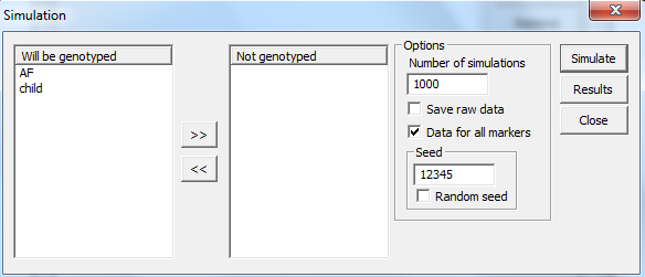
Figure 36. Starting a new
simulation. Selecting the individuals that will be/is genotyped and some other options.
The
above will give thousand simulations of AF and the child for all markers
defined, in this case only one. The seed set to 12345 so repeated simulations
will give the same results. The results appear in Figure 37. Below follows a description of the buttons
appearing in Figure 36.
Simulate
Start the simulations with the specified settings. Familias
may appear to “hang”/temporarily be unresponsive, but is in fact working hard
to complete the simulations. If mutations are considered, considerable
computation times can be expected.
Results
This will open the Results window, see Figure 37. The window will be opened automatically if a simulation process is
started.
Number of simulations
Specifies the number of simulations to be performed. It is
recommended to perform at least 1000 simulations to obtain reasonable values.
Keep in mind that for each simulation we will simulate data for each of the
pedigrees and do computations for all pedigrees. In other words, the total
number of computations will be #Simulations * #nPedigrees * #nPedigrees.
Save raw data
This will save the raw data from the simulations. Two
different types of data may be saved
1. Genotypes
2. Likelihoods
This is defined in the Advanced dialog.
Data for all markers
Default is on. This option allows the simulations to be
performed with either all markers in the frequency database or only the ones
selected in the Pedigrees dialog (see Included systems in Section
3.11)
Seed
Used to specify where the simulations will start. If the
same seed is used each time the simulations are started, we expect exactly the
same results, given all other values/parameters remain unchanged. Random seed
will use a different seed each time.
Will be genotyped
Specify which persons will be genotyped. In a case of
siblings (without data from the parents), the two siblings should appear as
genotyped while the parents should appear as not genotyped. The simulation will
then simulate data for all persons but only include genotypes for the siblings
in LR calculations.
Continuing
on our example, we have used a stepwise mutation model (stationary) and used
the Display button
to select the output in Figure 37.
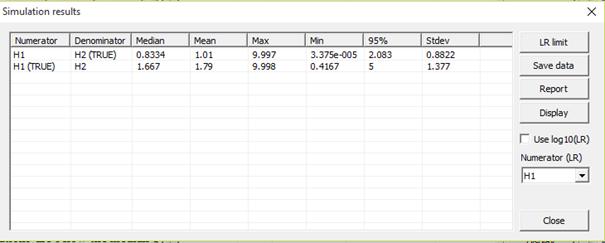
Figure 37. Simulation results
with summary statistics.
Consider the first line above. The simulations are
conditioned on H2 (denominator hypothesis), AF and child are unrelated. Data is
simulated for AF and child. We expect mostly small LR values, but not 0 as a
stepwise stationary mutation model with mutation rate 0.001 and range 0.1 is
used. 50% of the simulations are below the median 0.8334, the mean is 1.01. The
maximum value is 9.997. Line two gives the same result, but now conditioned on
that H1 is true, AF being the father and larger LR-s are expected, but not
hugely so as only one marker with four alleles is considered.
The LR limit button is used to find the fraction of
simulations exceeding a prescribed level, see figure below.
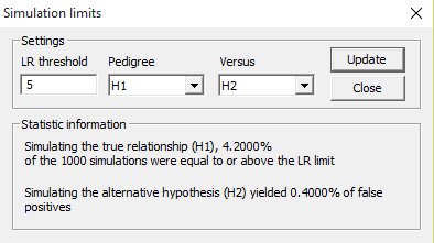
Figure 38. The simulation limit
window.
The buttons in Figure 37
is explained below.
LR limit
The dialog in Figure 38 appears. This is used to use
the simulation data to estimate true positive rate and false positive rate. In
other words, to display results in a way that may be easier to understand.
Save data
Save the output from the simulations (LR:s) The data can be
read into R after slight editing of the output file.
Report
Save a comprehensive report of the simulation results.
Display
Used to select which statistics to display.
If the Use
log10(LR) box is
ticked, all results are displayed on a logarithmic scale instead.
Further details on simulations are provided in Section 2.2
of Kling et al. (2014).
7
Familial searching
This section briefly describes functionality included in the
Familial searching module of Familias (version 3.1.6 and above).Familial
searching is a concept where we search a database of convicted offenders and
traces against reference profiles or traces from crime scenes to find
relatives. In other words, we compare each element of the database with each
profile of interest and compute a LR comparing the hypotheses that the two
profiles are related or not.
The interface is opened in Tools > Familial searching. The
action opens up the Import database dialog where the database of
persons/traces is defined. (Preferably imported from a file). Note, the
Familial searching interface can handle mixtures. The buttons appearing in Figure 39 is explained below.
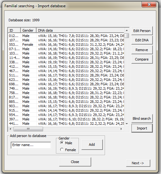
Figure 39. The Familias
searching interface - Importing database with convicted offenders.
Edit Person
Edit a person/database element
Edit DNA
Edit the DNA data of a selected person/database element.
Remove
Removes a selected person/database element
Compare
Compare the DNA data for a number of selected
persons/database elements. If only one person is selected, the random match
probability for the profile is displayed instead.
Blind search
Perform a blind search in the database. Find direct matches
and/or related elements.
Import
Import a database of persons/traces using any of the import
option described previously. It is common to have a CODIS database. The CODIS
format is the only allowing for the import of mixtures.
The next dialog is the Options dialog. The dialog a
combination of defining/importing the profiles/traces to search for and to
define the search parameters.
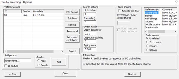
Figure 40. Familial searching interface – Defining
traces/profiles and search parameters.
Edit Person
Edit a person/trace
Edit DNA
Edit the DNA data of a selected person/trace
Remove
Remove a selected person/trace
Remove all
Remove all persons/traces
Set known
contributor
Set known contributors of a profile/trace. Used to e.g.
distinguish the profile of the perpetrator from the victim.
Import
Import a set of persons/traces using any of the import
options described previously.
LR threshold
Threshold for the a match to be reported, i.e. all matches
with a LR above the threshold will be saved for further processing.
Theta (Fst)
Correction for subpopulation effects. Positive value between
0 and 1.
Drop-in parameter
(Direct matching)
This function relates to the direct matching feature,
described in detail in Kling et al (2014). Briefly the drop-in parameter
describes the probability that an allele is in the profile as an artifact.
Dropout probability
(Direct matching)
This function relates to the direct matching feature,
described in detail in Kling et al (2014).Briefly the parameter describes the
probability that an allele has failed to amplify in the PCR, causing a
homozygote genotype, whereas the true genotype is heterozygote.
Typing error (Direct
matching)
This function relates to the direct matching feature,
described in detail in Kling et al (2014). Briefly the parameter describes the
probability that a genotype has been erroneously called in the analysis, also
known as any error caused in the laboratory procedure.
Activate IBS filter
Activates a filter that will remove matches that do not meet
the specified IBS thresholds, see below.
Percentage (%) of alleles shared
A filter that removes matches where the number of shared
alleles (total number shared IBS/total number possible shared for the
overlapping markers) is below this threshold.
Must share one allele per marker
Certifies that all matches share at least one allele per
marker
Relationships
Select the relationships to search for.
Scale versus
Select the relationship you wish the search to scale
against. Normally "Unrelated", unless there is a suspicion that the persons
in the database are related to some degree, e.g. in a smaller population individuals
may be related as 2nd cousins.
The next step is the Perfom search dialog, see Fel! Hittar inte referenskälla. below. An explanation of
the output is given at the end. Below follows a description of the buttons.
Figure 41. Familias searching interface –
Performing a search
Search
Perform a search using the specified parameters in the previous
dialog. The profiles/traces will be searched against all the database elements and
matches will be listed for all hits exceeding the LR threshold.
Sort
Sort the matches according to LR
Subset
Select a subset of the matches using specific methods.
Explanations are given for each method.
Display (Unused)
Select which things to display in the search window. Not
implemented yet.
View match
Brings up a window where the user obtains a detailed view of
the match with LR for each marker.
Report match
Create a report for a specific match.
Remove
Removes a selected match from the list.
Save summary
Save a summary of the search as a report
Export list
Export the search list to a tab-separated text file.
Explanation of the result
|
Profile/trace
|
Candidate
|
Index
|
Gender
|
|
The ID of the trace
|
The ID of the database
match
|
Index of the candidate in
the database
|
Gender of the candidate
|
|
Relationship
|
LR
|
Exclusions
|
|
The indicated relationship
for the candidate and the trace
|
The likelihood ratio given
the Relationship and the alternative hypothesis (usually unrelated)
|
The number of markers where
the trace and the candidate do not share any markers (only applies to
parent-child relationship)
|
|
Overlapping markers
|
Shared alleles
|
IBS=0,1,2
|
|
The number of overlapping
markers between the trace and the candidate
|
The percentage of shared
alleles.
|
Percentage of markers with
0,1 or 2 alleles shared IBS.
|
Some miscellaneous options are available by accessing File > Advanced,
see Figure 42 below.
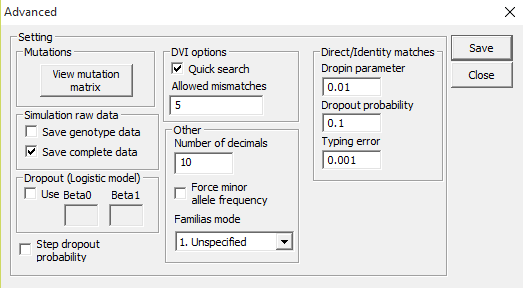
Figure 42. Advanced settings dialog.
View mutation matrix
The mutation matrix for a selected marker is displayed, see
figure below. The results can be exported to a tab-separated file using the Export
button.
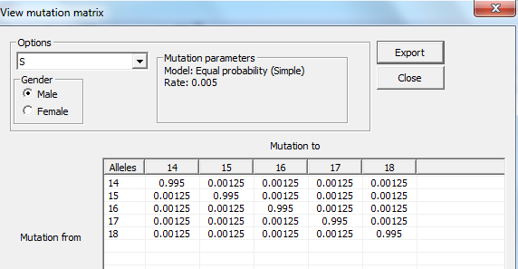
Figure 43. View mutation matrix dialog.
Simulation raw data
In connection with simulations (see Section 6), the user can specify that the simulation data is to be saved for potential
further use, e.g. plotting using other programs. The amount of data to be saved
(complete data or only genotype data) can be specified. Different default options
for names of output files are given depending on the choice of the user.
Dropout (logistic model)
Allelic dropout and its implication in relationship
calculations is described by Dørum et al (2015). The user may here select to
use profile specific dropout probabilities, instead of only marker specific.
A logistic model may be used to model dropouts. This option is
for advanced users only! We specify the model as:  , where d is the dropout
probability, H is the peak height of the surviving allele (measured in
RFU) and the β:s are estimated through regression, see for instance
STRvalidator, Hanson et al. (2015)
, where d is the dropout
probability, H is the peak height of the surviving allele (measured in
RFU) and the β:s are estimated through regression, see for instance
STRvalidator, Hanson et al. (2015)
Step dropout probability
Instead of specifying a static dropout probability the user may
desire to see the LR for a number of values. By ticking the Step dropout probability
feature, a dialog will appear when performing LR calculations asking the user to
specify a range of dropout probabilities.
Quick search
The quick search feature is implemented to perform a faster
search in the DVI module. If ticked, a fast search disregarding mutations will
be performed first. For matches with mutations (specifically markers where the
LR=0), calculations will be undertaken if the number of Allowed
mismatches is above the number of markers with LR=0. It is recommended
to allow quick searches for speed but setting the allowed mismatches fairly
high, e.g. 4-5 to allow for possible mutations. In other words, the allowed
mismatches corresponds to the number of inconsistencies we allow.
Number of decimals
The idea is that the user
can specify the number of digits (for floats) displayed in different windows,
e.g. the Pedigree window.
Force minor allele frequency
This options forces the minor allele frequency to be used in
LR calculations. (Only applies to computations in the Pedigree window.)
Be aware that by allowing this the sum of the allele frequencies for a
system/marker may exceed 1.
Familias mode
Specifies the project type, Normal (Casework), DVI
or Familial searching. Note that if selecting for instance DVI, only DVI
data will be saved.
Dropin parameter
Used in the direct
matching functionality, e.g. in DVI searches and blind searching. Specifies the
parameter used to assess the probability that an allele drops in.
Dropout probability
Used in the direct
matching functionality, e.g. in DVI searches and blind searching. Specifies the
probability that an allele drops out.
Typing error
Used in the direct
matching functionality, e.g. in DVI searches and Blind searching. Specifies the
probability that a genotype is typed wrong.
Feature will be described in detail in future versions of
the manual. Briefly, the feature is accessed in File > Create database. Fundamentally, the feature
can import genotype data for a number of individuals, for instance in the
GeneMapper format described in 3.9.1.3, without prior specification of a
frequency database. The functionality will create a database from these
individuals and produce some statistic information, such as important forensic
parameters. See Figure 44 below.
Figure 44. The create database tool
The feature is accessed in File > Export to R-Familias. This brings up the window
displayed below and lets the user export a complete Familias project to
the R version of the software. This includes functionality to plot the
pedigrees as well as the genotypes of the involved persons (requires the R library
paramlink to be installed). Further instructions appear on http://familias.name/openfamilias.html
and some useful links on http://familias.name/book.html.
The later versions of Familias (3.1.9.6 and above)
allows plotting of pedigrees. There are several ways to achieve this; they are
briefly described below.
1. Use
the software FamiliasPedigreeCreator, briefly mentioned in the Preface.
This software is freely available at http://www.familias.no
(Downloads section) and creates an R-script which in turn will create png files
for all Familias projects in a specified directory (and subdirectories).
The png files may then be displayed in the software via the Pedigrees
dialog and View Result button or inserted directly in a report.
2. Use
the option found in File > Export to R-Familias (Select
to plot). This will generate an R-script and plots will be displayed. These are
not automatically stored but the user can decide to if necessary.
3. Use
the option located in the Pedigrees dialog via Add/Edit
pedigree and the Plot button. This will generate an
R-script that can be run to plot the pedigree only. No files are stored.
4. In
the DVI module, either use the plotting function described in 3. to plot
individual pedigrees, or
5. Plot
all pedigrees using the function located in the Add Reference Families
window and the Prepare pedigree plots button. This will generate an
R-script that will plot and store the figures as png files (for all the
selected families). These can be displayed in the software by selecting the
same families and pushing the Evaluate button and in the next dialog
pushing the View Family button. The missing person will be indicated
with red.
There are several ways to alter the plots, we refer to the
R-package paramlink (https://cran.r-project.org/web/packages/paramlink/index.html)
implementing functions of the kinship2 package. A useful parameter is the cex
that will effectively increase or decrease the size and the text. Try
decreasing the parameter if the text/pedigree is to large, good values should
be 0.4-1.
This section contains some basic information about what
checks Familias performs to look for errors in input data (both files
and manual input). Here is a list of some common errors, remember the list is
not exhaustive. In addition, very little checking is performed on reading from
file.
|
Description
|
Handled
|
|
Input markers/systems
with an extra blank/space before or after the name
|
This is generally handled in Familias, but any
characters are otherwise accepted.
|
|
Input alleles with an
extra blank/space after or before the name
|
The same as above.
|
|
Names of
persons/individuals/pedigrees/families.
|
Duplicate names and empty names are not allowed.
Otherwise, all names are allowed with any characters.
|
|
Input numbers out of
bounds
|
Generally a check is performed to ensure all frequencies
or probabilities are in the range 0 to 1. Other numbers are normally checked
to be within reasonable ranges.
|
|
Relations
|
Generally whenever a relation is added to a pedigree or as
a known relation a check is performed to find if the relation is ok. Checks
include number of parents, gender of parents and year of birth of individuals
as well as some other consistency controls.
|
|
|
|
|
|
|
|
|
|
13 A Appendices
13.1 A1 Theory and
methods
The method Familias is based on may be divided into
the following stages: First, we describe the set of possible pedigrees
involving the relevant persons. This may sometimes be a very large number.
Secondly, we assign a prior probability distribution to this set of pedigrees,
based on non-DNA evidence. Finally, we introduce DNA measurements and mutation
parameters, obtaining a posterior probability distribution on the pedigree set.
Likelihood ratios (LR-s) may also be calculated and then prior distributions
are not needed.
Familias determines relationships between persons
through parent-child relations. When you define persons in Familias, you
distinguish persons based on those who may have children and those you know do
not have children. This distinction will typically be made based on age. It is
thus possible to define a person as a child. If no such information is
available, then the safest alternative is to classify all the persons as
adults. Next, the persons involved are characterized according to gender.
Based on the information above, one may generate all
possible pedigrees containing only these individuals. However, one will
frequently be interested in pedigrees involving persons not included in the
original group. For example, to describe that a woman has three children with
the same man, it is necessary to include this man in the pedigree, even though
his DNA is unavailable. The implemented approach introduces a number of “extra”
men and “extra” women and generates all possible, different pedigrees.
The set of pedigrees generated should contain the pedigrees
we consider probable given the background information, but will also contain a
large number of pedigrees that are unlikely for different reasons. For example,
many very incestuous pedigrees will be generated; in most cases, they should
not be considered a priori as likely as non-incestuous pedigrees. Similarly,
most pedigrees will indicate a more promiscuous behavior than is usual in most
cultures.
Familias generates a probability distribution on the
set of pedigrees reflecting such considerations. Starting with an equal
probability distribution on the pedigree set, we may choose to modify the prior
probabilities of different pedigrees using the three options inbreeding,
promiscuity and generations. The first parameter may be used to
increase or decrease the probabilitiesof pedigrees involving inbreeding. A
similar comment applies to promiscuity, while generations allude to the
modification of probabilities of pedigrees extending over several generations.
The prior distribution is proportional to

where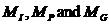 are non-negative parameters
provided by the user of the program. The subscripts refer to the three
mentioned options. The corresponding integer exponentials
are non-negative parameters
provided by the user of the program. The subscripts refer to the three
mentioned options. The corresponding integer exponentials  explained next are
calculated by Familias.
explained next are
calculated by Familias.  is the number of children whose
parents have a common ancestor in the pedigree. For promiscuity, the
number of pairs having precisely one parent in common is calculated and denoted
is the number of children whose
parents have a common ancestor in the pedigree. For promiscuity, the
number of pairs having precisely one parent in common is calculated and denoted
 . The number
of persons in the longest chain of generations starting with a named person and
ending in another named person is calculated and assigned the value
. The number
of persons in the longest chain of generations starting with a named person and
ending in another named person is calculated and assigned the value  . In addition, it is
possible to discard automatically all pedigrees where the number of generations
exceeds a
prescribed level.
. In addition, it is
possible to discard automatically all pedigrees where the number of generations
exceeds a
prescribed level.
Letting  , the prior probability of all
incestuous pedigrees is 0. A value of the parameter between 0 and 1 decreases
the probability of incestuous alternatives in comparison to non-incestuous
ones, while a value exceeding 1 increases the probability of incestuous
constellations. There is apriori no maximally incestuous pedigree as MImay
be arbitrarily large. Similar comment applies to the other options. A small,
artificial example illustrates some of the concepts above. Assume three men,
M1, M2 and M3 are found dead and two alternatives are considered: H1:
M1 is the father of M2 who is the father of M3 and H2: M1 is
the father of M2, while M3 is unrelated to M1 and M2. The ratio of the
priors corresponding to alternatives
, the prior probability of all
incestuous pedigrees is 0. A value of the parameter between 0 and 1 decreases
the probability of incestuous alternatives in comparison to non-incestuous
ones, while a value exceeding 1 increases the probability of incestuous
constellations. There is apriori no maximally incestuous pedigree as MImay
be arbitrarily large. Similar comment applies to the other options. A small,
artificial example illustrates some of the concepts above. Assume three men,
M1, M2 and M3 are found dead and two alternatives are considered: H1:
M1 is the father of M2 who is the father of M3 and H2: M1 is
the father of M2, while M3 is unrelated to M1 and M2. The ratio of the
priors corresponding to alternatives  and
and  follows from Equation (1) as
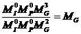
We emphasize that this prior is but one pragmatic suggestion
among many others possible; in many cases they are not needed. The default of
the parameters 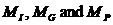 is
by Familias set to equal 1 and therefore implies that all pedigrees
have, a priori, the same probability. Further details on the prior model
including examples appear in Egelandet al. (2000).
is
by Familias set to equal 1 and therefore implies that all pedigrees
have, a priori, the same probability. Further details on the prior model
including examples appear in Egelandet al. (2000).
According to Bayes’ theorem the posterior probability
ratio (PPR) may be written as

In a more mathematical terminology
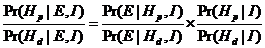
whereE typically stands for evidence, more precisely
DNA-data, and I is some conditioning information like for example age.
Relating to a forensic evidence interpretation, the term  is the prosecution
hypothesis and the defendant hypothesis is denoted
is the prosecution
hypothesis and the defendant hypothesis is denoted . Usually it is the likelihood
ratio (LR) that is reported in court.
. Usually it is the likelihood
ratio (LR) that is reported in court.
It remains to explain the calculation of the likelihood . A version of the
Elston-Stewart algorithm is implemented (Elston and Stewart 1971).
The algorithm is extended to account for possible substructure, silent alleles
and mutations and these extensions are explained in the coming sections.
. A version of the
Elston-Stewart algorithm is implemented (Elston and Stewart 1971).
The algorithm is extended to account for possible substructure, silent alleles
and mutations and these extensions are explained in the coming sections.
The probability of a set of DNA-data is calculated by
looking at the different loci separately before multiplying the results. For
all individuals, a locus of the DNA consists of two alleles, which can be
either equal, constituting a homozygous locus, or different, giving a
heterozygous locus. The probability of a particular combination of alleles (the
genotype) is in the simplest cases calculated by means of Hardy-Weinberg’s law.
This law states that the probability of being either heterozygote or homozygote
 is given by
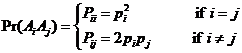
Wherepi is the frequency of allele Ai
in the population.
Assuming the following conditions are satisfied:
- random mating,
- no selection,
- no mutation,
- no migration,
the population in question is at so-called Hardy-Weinberg
equilibrium, and Equation (1.4) is valid.
In situations where mutations and non-random mating occur,
the assumptions in Hardy-Weinberg’s law are no longer necessarily satisfied. As mentioned, Hardy-Weinberg’s law may
not apply in the presence of population stratification and relatedness. To
handle this, Familias incorporates a kinship parameter, which is set by
the user. The parameter corresponds to the traditional FST
known from population genetics (see, e.g., [1]). It takes into consideration
that within a subpopulation there tends to be a higher frequency for
homozygosis than if Hardy-Weinberg equilibrium is obtained.
If  is the frequency of
  in the population,
then the genotypic frequencies are described by
in the population,
then the genotypic frequencies are described by
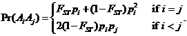
Generally, the complete correction (sometimes referred to as
-correction) described in (Balding and Nichols 1994)
is implemented.
The differences between probabilities calculated with and
without incorporating kinship can be quite large. For example, the probability
of a genotype (A, A) when pA = 0.05, is 0.00250.
However, using a kinship parameter of 0.01, this probability becomes 0.00298.
It can be problematic to decide an appropriate value for the
kinship parameter. One suggestion is to use 0.01-0.05 for Europeans while the
value may be even higher for more divergent populations.
There are fivedifferent mutation models available in Familias
(Egeland et al. (2000)). The mutation model is specified for each allele
system, and can be different for males and females. The alternative models are:
1)
Equal probability
(Simple)
2)
Probability
proportional to frequency (Stationary)
3)
Stepwise (Unstationary)
4)
Stepwise
(Stationary)
5)
Extended stepwise
(Unstationary)
We provide details of the models below in an order deviating
from the above for practical reasons.A mathematical note, the following section
requires an understanding of basic statistics and linear algebra.
A1.4.1 Step-wise
(unstationary).
It is convenient to first describe model 3. In the
decreasing model we assume that the list of alleles is expanded to include all
“possible” alleles, and that they are listed by increasing lengths. The
probability of mutation from allele a to allele b decreases in this model as a
function of the difference in length between the alleles. This property is
illustrated in Figure A.1, where the thickness of the arrows illustrates the
probability of the transitions. The transition matrix M for this model
is given by:
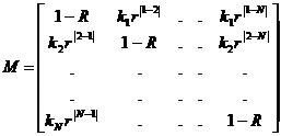 ,
,
WhereR is the overall mutation rate, r is a
constant between 0 and 1 (0<r<1). The r parameter is provided by
the user and is Mutation range
in Familias. ki is chosen such that  .
.
A calculation gives 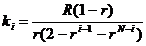 .
.
Figure A.1: Mutation
model
13.5.1 A1.4.2 Step-wise
(stationary)
This model is explained in(Dawid, Mortera et al. 2002)
and is a stationary version of the previously described model. Below we provide
some details beyond those presented in the mentioned paper. The current
implementation may give a somewhat unreasonable mutation matrix for some
particular combinations of parameter settings. We hope to rectify this problem
in future releases. In the meantime, the unstationary version may be a safer
version.
We want to generate stationary mutation models. Recall that
a mutation model can be represented as a square matrix  where
where  is the probability of mutating
from allele i to allele j. The fact that these values are
probabilities is contained in the requirement
is the probability of mutating
from allele i to allele j. The fact that these values are
probabilities is contained in the requirement  where 1 is the column vector
of ones, and in the requirement that all elements of M are non-negative.
Let p be the column vector of allele population frequencies and p’
the transposed(row) vector. Then M is stationary iff (if and only if) p’M
= p’
where 1 is the column vector
of ones, and in the requirement that all elements of M are non-negative.
Let p be the column vector of allele population frequencies and p’
the transposed(row) vector. Then M is stationary iff (if and only if) p’M
= p’
How can one modify a mutation model so that it becomes
stationary? Clearly this can be done in many ways, but an attractive
alternative would be to adjust, for each allele, the probability that a
mutation occurs, while keeping unchanged the relative probabilities of the
identities of the resulting mutated alleles after a mutation. In terms of a
mutation model matrix, this corresponds to adding (or subtracting) various
values along the diagonal, while adjusting the remaining values so that the
numbers on each line still sum to 1. Technically, let A be a mutation
model, i.e., A1 = 1 and all elements non-negative. Then we will find a
stationary version of it by writing M = DA + I – D, where D is a
diagonal matrix. We get
M1 = DA1 + 1 – D1 = 1, so M is a mutation
matrix, as long as D is defined so that the elements of M are
non-negative: This means that 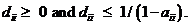 M
is also stationary iff p’M = p’, that is, if p’DA + p’ – p’D = p’,
i.e., iffp’DA = p’D, i.e., iffv = Dp is a right eigenvector of A’
belonging to the eigenvalue 1.
M
is also stationary iff p’M = p’, that is, if p’DA + p’ – p’D = p’,
i.e., iffp’DA = p’D, i.e., iffv = Dp is a right eigenvector of A’
belonging to the eigenvalue 1.
Assume A is symmetric, as it is in our examples. Then
1 is such an eigenvector, and we get a solution by defining D such that 1b
= Dp, where b is some positive scalar. Note that b must be
small enough so that

Thus we can always generate a stationary mutation model from
a symmetric mutation model matrix, in the manner above.
Define A by defining 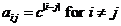 for some constant c, and
define
for some constant c, and
define for i=jso that
A1 = 1. Then the stabilized matrix M becomes defined by
for i=jso that
A1 = 1. Then the stabilized matrix M becomes defined by 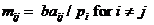 andfor i = jagain computed
so that M1=1. We get
andfor i = jagain computed
so that M1=1. We get
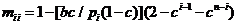
The parameter c is assumed input from biological
knowledge, while b is computed from the overall mutation rate R,
using the following relation:

giving
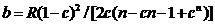
With the user giving as input R and c, the
program computes the mutation model M by first computing b as
above, then computing the off-diagonal elements of M, and then the
diagonal by requiring the rows to sum to 1. Note that the requirement that b
cannot be too large translates to the requirement that for all i
 .
.
As another example, define A = 1p’. then clearly A1
= 1. To stabilize it, we choose a D such that p’DA = p’D. We
may choose D = kI for some constant k. We get that we must have for all i, and, defining R
as above, we get that
for all i, and, defining R
as above, we get that
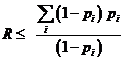
for all i.
A1.4.3 Extended step-wise model (unstationary).
The model is described in Kling et al. (2014) and a slightly
revised version appears below. There is a need for a new mutation model capable
of handling transitions to and from microvariants, e.g. between 9 to 9.3. Some
current models treat such microvariant mutations (MVM) in the same way
as integer mutations(IM) or neglect them as the mentioned transitions
are considered improbable. This is biologically unreasonable and the problem
has become more pronounced as MVM are more common in the latest STR kits.
We specify the model by letting M be the mutation
matrix, with elements mij, where i,j=1,…,N and where N
is the number of alleles. Each element mij is the probability
of a transition from allele Ai to allele Aj.
The current model separates the overall mutation rate, denoted  , into two parts, one
corresponding to integer mutations, R, and one to the micro-variants
, into two parts, one
corresponding to integer mutations, R, and one to the micro-variants , i.e.,
  Biologically R is often
explained by slippage error during DNA replication (Ellegren 2000)
while is connected to
insertions/deletions and point mutations. The last parameter, the mutation
range r, is defined as for previous IM models; it is the value with
which the probability decreases for each further step away from the original
allele mutates.
Biologically R is often
explained by slippage error during DNA replication (Ellegren 2000)
while is connected to
insertions/deletions and point mutations. The last parameter, the mutation
range r, is defined as for previous IM models; it is the value with
which the probability decreases for each further step away from the original
allele mutates.
Next the model is specified precisely by the transition
probabilities mij .There are three different alternatives:
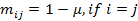 ,i.e. the probability that
an allele does not mutate.
,i.e. the probability that
an allele does not mutate.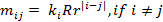 , for integer mutations.
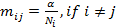 , for micro variant
mutations and Ni is the number of MVM-s from allele i.
, for micro variant
mutations and Ni is the number of MVM-s from allele i.
The rows must sum to unity and therefore the normalizing constants  are determined by the
constraints
are determined by the
constraints 
Example 1. Consider a marker containing the alleles
9, 9.3, 10, 10.3 and 15. The transition matrix M is then given by:
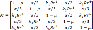
In this case, k1 is found as follows

Similar calculations can be shown for the other ki.
Note that, the matrix M is not symmetric, meaning that the probability of
observing a mutation from 9 to 9.3 is not the same as observing a mutation from
9.3 to 9. This is a consequence of the definition of M. Further note
that for transitions from allele 9 for example, Ni=2 as there
are two MVM:s given allele 9 as starting point. NB! There is a small deviation
of this model from the description that appears in Kling et al. (2014).
A1.4.4 Probability proportional to frequency (stationary)
In this model the probability of mutating to an allele is
proportional to that allele’s frequency. This model is as mentioned stationary.
The transition matrix M for this model is given by:
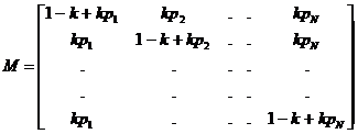
where is a constant. This model
satisfies the stationarity condition
is a constant. This model
satisfies the stationarity condition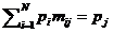 . The overall mutation rate
becomes
. The overall mutation rate
becomes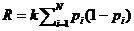 ,
therefore we must set the constant to be
,
therefore we must set the constant to be
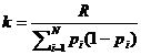 .
.
Note that if the frequency of the entered alleles do not sum
to 1, Familias will assume there is a single extra allele making up for
the rest of the probability when computing. If this is not the case, kwill be slightly wrong. Thus the
frequencies of all the alleles in the system should be entered when using the
proportional model.
13.5.2 A14.5 Equal
probability (simple)
In this model we assume that there are Q different
alleles observed in a database and that  is the number of “possible”
alleles. The model can best be described by means of a transition matrix M,
where the elements
is the number of “possible”
alleles. The model can best be described by means of a transition matrix M,
where the elements  denote
the probabilities that alleles
denote
the probabilities that alleles  are inherited as alleles
  (i, j = 1,…,N).
For this model, the probability of not mutating is for each allele
(i, j = 1,…,N).
For this model, the probability of not mutating is for each allele  , where R is
the overall mutation rate. The probability of mutating to any of the possible
other alleles is the same
, where R is
the overall mutation rate. The probability of mutating to any of the possible
other alleles is the same  . This model is in fact
stationary if and only if the allele probabilities are equal. So the transition
matrix M is given by:
. This model is in fact
stationary if and only if the allele probabilities are equal. So the transition
matrix M is given by:
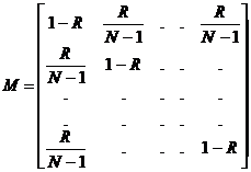
Note that the “frequency” of an allele entered into Familias
is in fact interpreted as the probability of observing that allele. Thus, if
the entered frequencies sum to 1, there is a zero probability of observing any
other alleles, and the program requires that . To use
  , you need to make
sure the probabilities input sum to (slightly) less than 1.
, you need to make
sure the probabilities input sum to (slightly) less than 1.
13.5.3 A1.4.6 An
example illustrating the mutation models
This example is a paternity case with an alleged father (AF)
with genotype (A, B) and a child (CH) with genotype (C, D).The
population properties of the allele system (S1) are given in Table A1.
Table A1: Properties of
allele system S1.
|
Allele label
|
A
|
B
|
C
|
D
|
E
|
F
|
G
|
H
|
|
Repeat
number
|
14
|
15
|
16
|
17
|
18
|
19
|
20
|
21
|
|
Count
|
44
|
49
|
127
|
175
|
133
|
58
|
12
|
2
|
|
Proportion
|
0.073
|
0.082
|
0.212
|
0.292
|
0.222
|
0.097
|
0.019
|
0.003
|
We consider the following hypotheses:
·
 :
AF is the father of CH.
:
AF is the father of CH.
·
:
AF and CH are unrelated.
We use a mutation rate of R = 0.005, and calculate
likelihood ratios assuming the various mutation models.
The likelihood assuming is . The likelihood assuming the
alternative hypothesis is
. The likelihood assuming the
alternative hypothesis is . So the likelihood ratio is
then
. So the likelihood ratio is
then
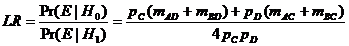
a) For
the equal probability model (model 1) we set the number of possible alleles to
8, which leads to .
The likelihood ratio then becomes
.
The likelihood ratio then becomes
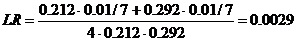 .
.
b) For
the proportional model (model 2) 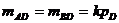 and
and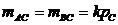 . Hence,
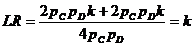 .
.
Furthermore, the constant is equal to
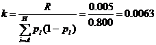 .
.
c) For
the decreasing model (model 3) we use a mutation range . The individual mutation
probabilities are
. The individual mutation
probabilities are
 ,
,
where
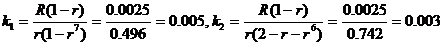 .
.
This leads to

d) For model
4, we calculate , matrices A
and Mas explained in Appendix 4.2 and find
, matrices A
and Mas explained in Appendix 4.2 and find

The different models lead to very small likelihood ratios as
expected. However, the relative differences are considerable and the choice of
model might well influence the overall LR considerably. Usually it will be a
good idea to check the robustness of the conclusions by incorporating different
mutation models.
13.6 A2 Solved excercises
The Familias 2.0 (or 1.97) exercises remain available
from http://familias.name.
New exercises with solutions for Familias 3 are now available from http://familias.name/book.html
13.7
A3 Generating pedigrees automatically
The Generate
button of the Pedigrees
window can be used to generate pedigrees automatically. All possible pedigrees
involving parent child relationships are generated. Keep in mind that as more
persons are introduced, the number of generated pedigrees increases almost
explosively. Often, as in the cases where only two pedigrees are to be
compared, it is preferable to construct them manually. So far the largest
number of pedigrees generated in a case is about 10000 (in test examples).
There is no limit to the number of pedigrees produced, however, extreme cases
may cause the program to “hang” [2].
When generating pedigrees, the program uses the information
that some persons are designated as children (i.e., having no children) and the
Year of Birth information. No pedigrees will be generated that imply a
generation length of less than 12 years. The generated pedigrees are named
Ped1, Ped2, … etc. To view the details of a pedigree, double-click it; and the
window in the figure below appears.
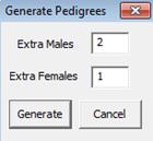 This is the same
window that appears when pressing Add
for manual construction of pedigrees. The pedigree is defined by the
list of parent-child relations, and is thus altered by adding or removing these
relations. You use the Persons-button
to add the extra men and women that are necessary to define the wanted
pedigree.
This is the same
window that appears when pressing Add
for manual construction of pedigrees. The pedigree is defined by the
list of parent-child relations, and is thus altered by adding or removing these
relations. You use the Persons-button
to add the extra men and women that are necessary to define the wanted
pedigree.
Figure A1.Adding extra persons.
As an alternative to adding anonymous extra persons here,
the extra persons could have been defined in the Persons
window described above. This is especially useful if one wants to put
constraints on the number and types of possible pedigrees generated
automatically, by introducing, e.g., extra persons that are of a certain age.
Note that this may influence the computation of the Generationsparameter.
13.8 A4 Implementation of
prior distribition
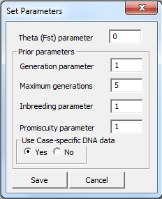
Figure A2 Parameter settings
After having entered the interesting pedigrees, one can
calculate posterior probabilities for the various alternatives. By pressing Parameters(see Figure 20), the window shown in Figure A2 appears. Here you are supposed to specify
parameters that are used in the calculations of posterior probabilities,
including the parameters defining the prior. The default corresponds to a
non-informative prior, that is, where all the pedigrees get the same prior
probability. After a possible change in the parameters the pedigrees’ posterior
probabilities appear. The pedigrees are now listed by decreasing probability.
The Generations
parameter gives you the opportunity to modify the likelihood of
pedigrees extending over several generations. More precisely, the calculated
number is the number of persons in the longest chain of generations starting
with a named person (not an “extra” person) and ending in an adult (not a
“child”). For example, a pedigree consisting of a father and an adult son has
generations value  ,
while if the son is marked as “child”, the generations value is
,
while if the son is marked as “child”, the generations value is  . By setting the
generations parameter to a number between 0 and 1, short pedigrees are
emphasized, and by using a number larger than 1, long pedigrees are
emphasized. In addition, it is possible to define a cut-off length for the
generation chain. By specifying Max
generations to, e.g., 2, you give a prior probability of zero to all
pedigrees extending over more than two generations.
. By setting the
generations parameter to a number between 0 and 1, short pedigrees are
emphasized, and by using a number larger than 1, long pedigrees are
emphasized. In addition, it is possible to define a cut-off length for the
generation chain. By specifying Max
generations to, e.g., 2, you give a prior probability of zero to all
pedigrees extending over more than two generations.
The Inbreeding
parameter is used to alter the prior probability of incestuous
pedigrees. More precisely, the value computed is the number of
persons in the pedigree such that its parents have a common ancestor. Thus, for
example, a pedigree where cousins have three children together gets a value  , while one where
siblings have one child gets a value
, while one where
siblings have one child gets a value  . Setting the inbreeding
parameter to zero is equivalent to giving a zero prior probability to all
incestuous constellations. A value between 0 and 1 decreases the prior
probability of incestuous alternatives relative to the non-incestuous ones,
while a value exceeding 1 increases the probability of incestuous
constellations.
. Setting the inbreeding
parameter to zero is equivalent to giving a zero prior probability to all
incestuous constellations. A value between 0 and 1 decreases the prior
probability of incestuous alternatives relative to the non-incestuous ones,
while a value exceeding 1 increases the probability of incestuous
constellations.
The Promiscuity
parameter is used to alter the prior probability of pedigrees involving
“promiscuous” behavior. More precisely, the value  computed is the number of pairs
of half-siblings. Again: a value between 0 and 1 suppresses such pedigrees,
while a value superseding 1 enhances them. Setting the parameter to zero gives
a zero prior probability to all pedigrees where any person has children with
more than one partner.
computed is the number of pairs
of half-siblings. Again: a value between 0 and 1 suppresses such pedigrees,
while a value superseding 1 enhances them. Setting the parameter to zero gives
a zero prior probability to all pedigrees where any person has children with
more than one partner.
Example: Given the pedigree in Figure A3 and
parameters provided by the user MG = MI =
MP = 0.5. The program will evaluate the pedigree and calculate
the corresponding b – factors, which in this case are bG=
3, bI= 3 and bP= 3, giving a value
 .
(Note that each of the children are half-siblings with their mother, giving
.
(Note that each of the children are half-siblings with their mother, giving  ). This means that
this pedigree will be weighted down in comparison to a pedigree where the
generations-, inbreeding- and promiscuity-factors are smaller, giving the
pedigree in Figure A3 a smaller prior.
). This means that
this pedigree will be weighted down in comparison to a pedigree where the
generations-, inbreeding- and promiscuity-factors are smaller, giving the
pedigree in Figure A3 a smaller prior.
You may choose to calculate the posterior probabilities without
the use of case-specific DNA data, by selecting “No” for the relevant variable.
This will show you the prior probability distribution on the pedigrees, and is
useful whenever you use a non-flat (non-default) prior.
The Kinship
parameter takes values between 0 and 1.

13.8.1
Figure A3: Pedigree
By pressing OK
in the Probability-window,
the posterior probabilities for all pedigrees appear, and the list is also
sorted from the most probable to the least probable pedigree.
13.8.2
Note that, when computing probabilities, the program will
remove all pedigrees found to be equivalent to a previous pedigree in the list.
For example, if the user has entered the pedigree without any relationships
several times, only the first of these will remain.
13.9 A5 Description of
general input files for Familias
The purpose of this document is to enable programmers to
write code producing input files for the Familias program, on the “Familias
format”. This format was designed to store all information contained in the
user interface between runs of Familias. Thus it was never designed to be
readable or practical to use as a data exchange format. Nevertheless, it is
released now as possibly the simplest way to exchange data between Familias and
other computer applications.
13.9.1 Versions
The Familias format can often change for each release.
However, backwards compatibility is ensured in that any version of Familias is
able to read the format output from all previous versions. The key here is that
the version number of the program producing the file is always given in the third
line of the file. The format described in this document is the one output from
version 1.81. Thus it will not be readable by previous versions of Familias.
But it will be readable by future versions.
13.9.2 Simplified
format
The “Familias format” stores some information which is
irrelevant when importing data from other programs in order to do computations
with Familias. For example, it is possible to store already computed
probabilities, or the order in which pedigrees are listed in the pedigree list.
In the table given below, lines specifying such information have been
simplified and set to default values. However, the completely general use of
these lines is explained in the notes below the table.
13.9.3 Format
verification
As the format was not really intended to be produced by
other programs, very little verification is done at the input stage that the
input file really conforms to the correct format. For example, it is not
checked that indices of persons and alleles are within the bounds given by the
sizes of the lists, that pedigrees are legal as pedigrees, and so on. Run-time
errors, or even faulty results, are likely to occur if the input files are
incorrect.
13.9.4 How
to interpret the table
The table below has four columns. The first contains line
numbers: These are included for reference only; the actual format does not
contain such numbers. The second column describes the information each line
should contain. Information inside comparison signs,
<like this >
is meta-information, and should be substituted with the
corresponding content. Information without such signs should be included as
written.
The third and fourth columns of the table indicate which
lines should be repeated, and how they should be repeated.
13.9.5 File
format
|
1
|
<Any text, in quotes; may describe the file >
|
|
|
|
2
|
<Any text, in quotes; may describe the file >
|
|
|
|
3
|
1.81
|
|
|
|
4
|
< Number of persons involved in pedigrees >
|
|
|
|
5
|
<Name of person >
|
|
}
}
} Repeated
} for each
} person
}
}
}
}
|
|
6
|
#FALSE#
|
|
|
7
|
-1
|
|
|
8
|
#FALSE#
|
|
|
9
|
<#TRUE# if male, #FALSE# if female >
|
|
|
10
|
< Number of allele systems with data for this person
>
|
|
|
11
|
< Index of first allele, starting at zero >
|
} Repeated
} for each
} allele system
|
|
12
|
< Index of second allele, starting at zero >
|
|
13
|
< Index of system, starting at zero >
|
|
14
|
< Any text , in quotes>
|
|
|
|
15
|
0
|
|
|
|
16
|
0
|
|
|
|
17
|
0
|
|
|
|
18
|
< Number of pedigrees >
|
|
|
|
19
|
< Index of pedigree, starting at 0 >
|
|
}
}
} Repeated
} for each
} pedigree
}
}
|
|
20
|
< Name of pedigree >
|
|
|
21
|
0
|
|
|
22
|
0
|
|
|
23
|
< Number of relations in pedigree >
|
|
|
24
|
< Index of parent in relation, starting at zero >
|
} Repeated for
} each relation
|
|
25
|
< Index of child in relation, starting at zero >
|
|
26
|
#FALSE#
|
|
|
|
27
|
< Number of allele systems >
|
|
|
|
28
|
#FALSE#
|
|
|
|
29
|
< Name of allele system, in quotes >
|
|
}
}
}
}
}
} Repeated
} for each
} allele
} system
}
}
}
}
|
|
30
|
< Female mutation rate >
|
|
|
31
|
< Male mutation rate >
|
|
|
32
|
< Female mutation model >
|
|
|
33
|
< Male mutation model >
|
|
|
34
|
< Number of possibilities >
|
|
|
35
|
< Female mutation range >
|
|
|
36
|
< Male mutation range >
|
|
|
37
|
< #TRUE# or #FALSE#: system has a silent allele >
|
|
|
38
|
< Silent allele frequency >
|
|
|
39
|
< Number of alleles in the system >
|
|
|
40
|
< Allele name >
|
} Repeated for
} each allele
|
|
41
|
< Allele frequency >
|
13.9.6 Explanation
by line numbers
|
LINE NUMBERS
|
EXPLANATION
|
|
1-2
|
We encourage that the first two lines are used to describe
the program producing the file. They are not read by the familias program.
|
|
3
|
The version number for the format: The file will be
readable by familias with a version number higher than or equal to this
number.
|
|
4
|
In the simplified format, we assume that all persons
involved in the pedigrees have a name, and are listed in the list of persons
further down. However, in general in familias, some pedigrees could be
described using “extra persons” without names. These persons would then not
be included in the total number of persons given on this line.
|
|
5
|
The name should be given in quotes, like “Mother”.
|
|
6
|
This line should be #TRUE# if year of birth data is
included for this person, otherwise it should be #FALSE#. Note that familias
uses the year of birth for a person only when automatically generating new
pedigrees, so it should rarely be necessary to input such information.
|
|
7
|
When the previous line is #FALSE#, this line should
contain -1. Otherwise, it should contain the year of birth for the person.
|
|
8
|
This line should be #TRUE# if the person is specified as a
“child”, otherwise, it should be #FALSE#. The default value is #FALSE#. Note
that familias only uses this information when automatically generating new
pedigrees, so it should rarely be necessary to use anything but the default
setting here.
|
|
10
|
Persons included just to describe the pedigrees properly,
and for which no DNA data is available, should have 0 here. Note that it is
not necessary that all the persons who do have DNA data have data from exactly
the same allele systems.
|
|
11
|
The index of the first allele for this person in this
allele system should be given: It is the index (when counting from zero) of
the allele in the list of alleles for this system given further down in the
file.
|
|
12
|
The index of the second allele; see line 11. Note that
even homozygote persons must be input with two (equal) alleles.
|
|
13
|
The index of the allele system in which the two alleles
above are contained: It is the index (when counting from zero) of the allele
system in the list of such systems given further down in the file.
|
|
14
|
This line will generally contain the text “Known
relations” in files produced by familias: The line is not used when reading
in data.
|
|
15 - 17
|
In general, these lines are used to specify fixed
relations, i.e., relations which occur in all pedigrees. In our simplified
format, we assume that all relations are specified directly in the pedigrees.
Thus these lines should just contain zeroes. In general, the format is as
follows:
Line 15 contains the number of “extra females” used to
specify the fixed relations. Line 16 contains the number of “extra males”.
Line 17 contains the number of fixed relations. Then follow pairs of lines,
with one pair for each relation. The first line of each pair specifies the
index of the parent of the relationship, and the second line the index of the
child. The indices start at zero in the list of available persons: This list
starts with the list of named persons, continues with the extra females, and
ends with the extra males.
|
|
18
|
The number of pedigrees. For most applications, this
number should be 2.
|
|
19
|
In our simplified format, this should just be 0 for the
first pedigree, 1 for the second pedigree, and so on. In general, these
numbers are used for the following purpose: The order in which the pedigrees
are listed in the pedigree window can change after probabilities are
computed; then they are listed by decreasing probability. When a familias
file containing already computed probabilities is stored, the line indicates
the place (starting at zero) of this pedigree in that ordered list.
|
|
20
|
The name of the pedigree. The name should be included in
quotes, like “Ped1”. The actual name can be chosen freely, as long as two
pedigrees do not have identical names.
|
|
21
|
This indicates the number of “extra females” in the
pedigree, i.e., females that are included the pedigree in order to describe
it correctly, but for whom we have no DNA data. For most applications, we
would recommend using named persons instead, and include these in the list of
persons above.
|
|
22
|
The number of “extra males” in the pedigree: See line 21.
|
|
23
|
The number of relations in the pedigree.
|
|
24
|
The index (when counting from zero) of the parent in the
relation, in the list of persons given above. When “extra persons” are
included, the list is extended, first with the extra females, and then with
the extra males.
|
|
25
|
The index (when counting from zero) of the child in the
relation, in the list of persons given above. When “extra persons” are
included, the list is extended, first with the extra females, and then with
the extra males.
|
|
26
|
This line should be #TRUE# when already computed
probabilities are included in the file. The default is #FALSE#. If computed
probabilities are included, a number of lines are inserted between lines 27
and 28: For each pedigree, the following is listed: First the probability for
the pedigree, and then, with one line for each allele system, the likelihood
for the data in this system with this pedigree. Then follows a line with
#TRUE# or #FALSE# according to whether DNA data was used to compute the
probabilities (i.e., whether they are prior or posterior probabilities), a
line with the kinship parameter used in computations, and finally lines
specifying each of the following parameters used in the computations: The
generations parameter, the max generations parameter, the inbreeding
parameter, and the promiscuity parameter.
|
|
27
|
The number of allele systems
|
|
28
|
This should be #TRUE# if “database information” is
included in the data. The default is #FALSE#. (This line is NOT repeated for
each allele system.) If database information is included, an extra line is
inserted below this line: It contains, in quotes, the string specifying the
database information. (This is the string specified in the top field of the
“General DNA data” box of the user interface).
|
|
29
|
The name of the allele system, in quotes, like “Allele
system”. Note that the name can be anything, but that different allele
systems must have different names.
|
|
30-31
|
These are the female and male mutation rates; default is
0. The numbers must be non-negative and less than 1. If the mutation model is
1 or 3, there are also some (high) theoretical limits to how high the
mutation rate can be; consult the manual for details.
|
|
32-33
|
Indices in the list of possible mutation models:
0 means “Equal probability (simple and fast)”
1 means “Probability proportional to frequency
(stationary)”
2 means “Prob. decreasing with range (equal)”
3 means “Prob. decreasing with range (stationary)”
Default is 3.
See the allele system window in the user interface, and
the manual, for further explanation.
|
|
34
|
The total number of alleles, including the silent allele.
|
|
35-36
|
The “range” of the mutation model: This is the same number
that is input in the corresponding box in the user interface. It must be a
positive number less than 1. For more detailed information, consult the
manual. Default is .1.
|
|
37
|
Use #TRUE# if the system has a silent allele, use #FALSE#
otherwise.
|
|
38
|
When there is no silent allele, use 0 as a default;
otherwise use the frequency of the silent allele.
|
|
39
|
The number of alleles in the system, NOT including a
possible silent allele. There must be at least 2 alleles in each system.
|
|
40
|
The name of the allele, in quotes, like “A1”. Note that
the names can be anything, but that different allele systems must have
different names. Note also that for mutation models 2 and 3 (se lines 32-33)
the order of the alleles matter. Thus the alleles are always assumed to be
ordered alphabetically, and should be input in alphabetical order.
|
|
41
|
The frequency of the allele. Note that the frequencies of
alleles in a system, including any silent allele, must add up to exactly 1.
All frequencies must be positive numbers.
|
Balding, D. J. (2005). Weight-of-evidence for Forensic DNA
Profiles, John Wiley & Sons.
Balding,
D. J. and R. A. Nichols (1994). "DNA profile match probability
calculation: how to allow for population stratification, relatedness, database
selection and single bands." Forensic Sci Int64(2-3): 125-140.
Bennett, R. L., K. S. French, et al. (2008).
"Standardized human pedigree nomenclature: update and assessment of the
recommendations of the National Society of Genetic Counselors." Journal
of genetic counseling17(5): 424-433.
Buckleton,
J. S., C. M. Triggs, et al. (2005). Forensic DNA evidence interpretation,
CRC Press.
Dawid, P. A., J. Mortera, et al. (2002).
"Probabilistic Expert Systems for Forensic
Inference from
Genetic Markers." Sand J of Statistics29(4): 577-595.
Drabek,
J. (2009). "Validation of software for calculating the likelihood ratio
for parentage and kinship." Forensic Science International: Genetics3(2):
112-118.
Egeland,
T., D. Kling, et al. (2015). Relationship Inference with Familias and R:
Statistical Methods in Forensic Genetics, Academic Press.
Egeland, T., P. F. Mostad, et al. (2000). "Beyond
traditional paternity and identification cases. Selecting the most probable
pedigree." Forensic Science International110(1): 47-59.
Ellegren,
H. (2000). "Heterogeneous mutation processes in human microsatellite DNA
sequences." Nature Genetics24(4): 400-402.
Elston, R. C. and J. Stewart (1971). "A general model for
the genetic analysis of pedigree data." Hum Hered21(6):
523-542.
Kling, D. and S. Füredi (2016). "The successful use of
familial searching in six Hungarian high profile cases by applying a new module
in Familias 3." Forensic Science International: Genetics24:
24-32.
Kling, D., A. O. Tillmar, et al. (2014). "Familias
3-Extensions and new functionality." Forensic Science International:
Genetics13: 121-127.